Inverse modeling for atmospheric trace gas inversions describes the statistical estimation of emissions given a set of atmospheric concentration data. By measuring the composition over time and knowing how material is transported through the atmosphere, we can estimate the emissions that would be required to produce that time-series of data.
In order to “invert” concentration data into emissions, we need a model of atmospheric transport and chemistry. This model, which is based on the physics of atmospheric dynamics, provides us with quantitative information of how air has been circulated around the globe. This essentially links “emissions” with “concentrations.”
The traditional inverse method used in most trace gas inversions is Bayesian, which uses information from the data as well as information from a “prior” set of knowledge about these emissions. This a priori information is used to condition the system, as most often, the system is underdetermined, or has more unknowns than data. We typically get this prior from databases that catalog emissions from “bottom-up methods.” For example, a bottom-up method for CH4 from cattle might involve conducting a census of cattle and using measurements from a small sample of these cattle to compute an emissions factor (that is, how much CH4 released per cattle). These factors then scale up the entire cattle population. While this is prone to large errors, due to the variability of emissions factors from cattle to cattle, or region to region), this databases can provide valuable information on the distribution of emissions around the world and provide a first-guess at what the emissions might be. We then use our atmospheric data to refine this first-guess.
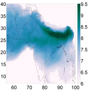
I am currently using the UK Met Office’s Lagrangian Particle Dispersion Model (LPDM), Numerical Atmospheric dispersion Modeling Environment (NAME), to produce maps that contain the sensitivity of measured concentrations to surface emissions, which is directly the sensitivity matrix required to invert for emissions.
