One of the main issues in trace gas inversions is in being able to correctly quantify the uncertainties in the system, as the inversion is very sensitive to these parameters. These errors include a complete understanding of uncertainties in the instrument, uncertainties in the model and uncertainties in the a priori emissions. In practice, being able to quantify these uncertainties is almost impossible.
To reduce the effect of errors in the assumptions made about these uncertainties, we have published a paper in Atmospheric Chemistry and Physics that details a hierarchical Bayesian inversion framework. This framework is used to deduce time-varying uncertainties and correlation parameters.
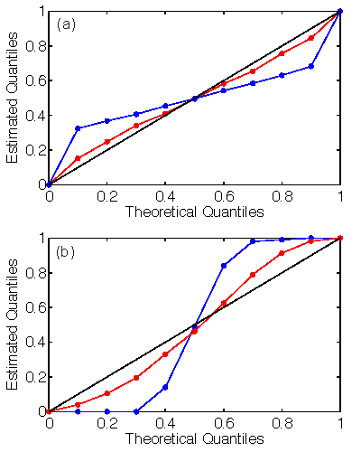
We show that the hierarchical method results in a more complete characterization of uncertainties, as shown by quantile-quantile plots blow. To interpret these plots, a Q-Q plot on the 1:1 line means that the error statistics of the inversion are correctly capturing uncertainties in the system. A Q-Q plot that is either an inverted S-curve or an S-curve indicates that the uncertainties specified in the inversion are under-constrained or over-constrained (that is the quantiles are either being over or under represented). We show that inclusion of additional parameters in the inversion to accommodate “uncertainty in these uncertainties” results in a Q-Q plot that shifts toward the 1:1 line.
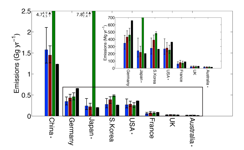
In our paper, we show how the hierarchical system can lead to more accurate emissions estimates. We present case study of sulfur hexafluoride emissions, and specifically highlight East Asian emissions derived with different estimates of model uncertainty. The differences are considerable, and emphasizes the importance of characterizing uncertainties properly.